See also Roll-out utility if you don’t want to get a vector utility over all states.
solving for the utility of a policy
We can solve for the utility of the policy given the transitions \(T\) and reward \(R\) by solving the following equation
\begin{equation} \bold{U}^{\pi} = (I - \gamma T^{\pi})^{-1} \bold{R}^{\pi} \end{equation}
where \(T\) is an \(|S| \times |S|\) square matrix where each horizontal row is supposed to add up to \(1\) which encodes the probability of transitioning from each horizontal row to the column next rows.
lookahead equation
We begin our derivation from finite-horizon models.
Gives some policy \(\pi\), at the base case:
\begin{equation} U^{\pi}_{1} (s) = R(s, \pi(s)) \end{equation}
at time \(k+1\) steps remaining:
\begin{equation} U^{\pi}_{k+1}(s) = R(s, \pi(s)) + \gamma \sum_{s’} T(s’ | s, \pi(s)) U^{\pi}_{k} (s’) \end{equation}
we don’t know what the next state will be; so for each possible next state, we marginalize the result, multiplying the probability of being in that state (gotten by \(T(…)\)) times the utility of being in that state.
This is called the lookahead equation, which represents how much utility any future state can be be if we took action at point \(k\).
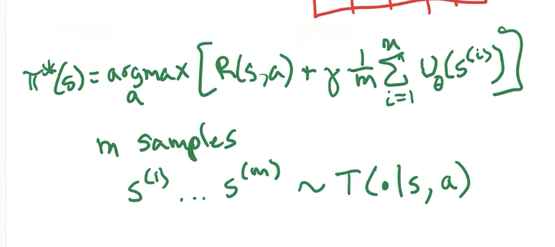
lookahead with sampling
what if we only want to get \(m\) of the next states, instead of all next states?

Bellman Expectation Equation
The Bellman Equation states that “the expected utility of being in a state is the instantaneous reward of being in that state plus the discounted future utility of all possible future state.” It is the fundamental result of RL.
\begin{equation} U(s) = \arg\max_{a} R(s, a) + \gamma \sum_{s’} T(s’ | s, a) U (s’) \end{equation}
If we are dealing with infinite-horizon models (at “convergence” of the lookahead equation), we just no longer have a time dependency from the lookahead equation:
We only care about some Markovian state \(s\), and its next possible states \(s’\). When these pair happened doesn’t matter.
For a stochastic policy, we have:
\begin{equation} U(S) = \sum_{a}^{} \pi(a|s) \qty[R(s,a) + \gamma \sum_{s’}^{} T(s’|s,a) U(s’)] \end{equation}
We now can go about solving for what \(U^{\pi}\) is:
Procedure:
from the Bellman Expectation Equation, we actually have a linear equation whereby:
\begin{equation} \bold{U}^{\pi} = \bold{R}^{\pi} + \gamma T^{\pi}\bold{U}^{\pi} \end{equation}
where, \(T^{\pi}\) is an \(n\times n\) matrix where \(T^{\pi}_{i,j}\) represents the probability of transitioning from the \(i\) th to the \(j\) the state; and where, \(\bold{U}^{\pi}\) and \(\bold{R}^{\pi}\) are \(n\) vectors which represents all possible states and all possible utilities. Note that everything is parametrized on \(\pi\) (so \(T\) doesn’t need an action dimension because we will be using the policy to calculate all the actoins)
We can now solve for the utility of the policy. Now, algebra time on the previous equation to get us:
\begin{equation} \bold{U}^{\pi} = (I - \gamma T^{\pi})^{-1} \bold{R}^{\pi} \end{equation}
we know that \(T\) is invertable because its a transition matrix. And that, folks, is the utility of a policy.
Approximate Policy Evaluation
Instead of having a policy evaluation based on a vector out of the fitness of this policy at all possible states, which really works if our state space is small, what if we made a policy evaluation scheme which estimates the expectation of the utility of our policy based on the possibility of us landing in particular states?
Background
The utility from following a policy AT A STATE is given by:
\begin{equation} U^{\pi}(s) = R(s, \pi(s)) + \gamma \sum_{s’} T(s’ | s, \pi(s)) U^{\pi} (s’) \end{equation}
The utility of a policy, in general, can be represented by:
\begin{equation} U(\pi) = \sum_{s}^{} b(s) U^{\pi}(s) \end{equation}
where, \(b(s)\) is the “initial state distribution” of being in a particular state.
Our state space may not be discrete or otherwise small enough to be added up for every case. We therefore can a sampling of Rollout trajectory to perform Approximate Policy Evaluation
Rollout utility
Collecting a utility for all \(s\) is real hard. Therefore, instead, we perform a bunch of Rollouts and then calculate, for each trajectory \(\tau\) you ended up with:
\begin{align} U(\pi_{\theta}) &= \mathbb{E}[R(\tau)] \\ &= \int_{\tau} p_{\tau} (\tau) R(\tau) d\tau \end{align}
where, \(p(\tau)\) is the probability of that trajectory happening, and \(R(\tau)\) is the discounted future reward of that trajectory. That is:
\begin{equation} R(\tau) = \sum_{k=1}^{d} r_{k}\ \gamma^{k-1} \end{equation}
monte-carlo policy evaluation
Sometimes, we can’t even get all trajectories to add them up, so we simply perform an average of \(m\) sample trajectories:
\begin{equation} U(\pi_{\theta}) = \frac{1}{m}\sum_{i=1}^{m} R(\tau^{i}) \end{equation}
We start each trajectory using a probability-weighted sample of initial states. This is the Roll-out utility