Metric
Sometimes we can just get a specification easily from just a metric, like (“the aircraft can’t be more than 50 meters apart”)
value at risk
see value at risk
composite metrics
weighted sum method
depends on how you care about each value, perform weighted sum and optimizes over a single metric \(\sum_{i=1}^{n} w_{i}f_{i}\qty(\tau) = w^{T}f\qty(\tau)\)
But, coming up with the weights is a bit hard! So we get them by asking pairwise questions with Preference Elicitation
goal distance metric
pick a Utopia Point, and find distances from that point \(\norm\mid f\qty(\tau) - f_{\text{goal}} \norm_{p}\)
logical specification
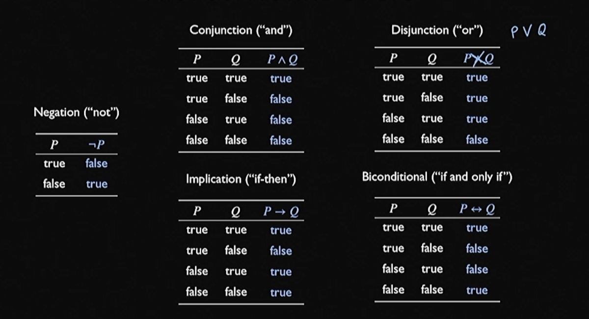
propositional logic
a proposition is a statement that evaluates to either true or false; an atomic proposition is a proposition that can’t be broken down further.
For instance, consider “not”:
example
“If the agent is in \(S\), then agent is not in \(C\)”
\begin{equation} S \to \neg C \end{equation}
first-order logic
First order logic adds variables, predicates, and quantifiers to propositional logic.
- predicate: a function that evaluates propositions over variables
- variables: objects in a domain
- quantifiers: evaluate propositions over a collection of variables
- universal quantifier: allows us to evaluates propositions over a collection of variables \(\forall\)
- existential quantifier: allows us to evaluate positions over any one of the variables \(\exists\)
example
variables: state \(x\)
predicates
\begin{equation} O(x): x \text{ is an obstable} \end{equation}
\begin{equation} G(x): x \text{ is an goal} \end{equation}
“an agent must reach a goal state and avoid the obstacle state
\begin{equation} \qty(\forall x \neg O\qty(x)) \wedge \qty(\exists x G(x)) \end{equation}
temporal logic
temporal logic specifies logic in time
linear temporal logic
always:
\begin{equation} \square P \end{equation}
this means “\(P\) is true at all time stamps in the future (including the current timestamp)”
eventually:
\begin{equation} \lozenge P \end{equation}
this means “\(P\) is true at some timestamps in the future (including the current timestamp)”
until
\begin{equation} P \mathcal{U} Q \end{equation}
“\(Q\) is true at some timestamp in the future and \(P\) is true at least until \(Q\) becomes true”
this lasts the lifetime until \(Q\) becomes no longer true.
example
“eventually reaches the goal after passing through the checkpoint and always avoids the obstacle”
Three predicates: \(F\) the obstacle, \(G\) the goal, \(C\) the checkpoint
\begin{equation} \lozenge G \wedge \neg G \mathcal{U} C \wedge \square \neg F \end{equation}
signal temporal logic
signal temporal logic extends linear temporal logic to real-valued signals
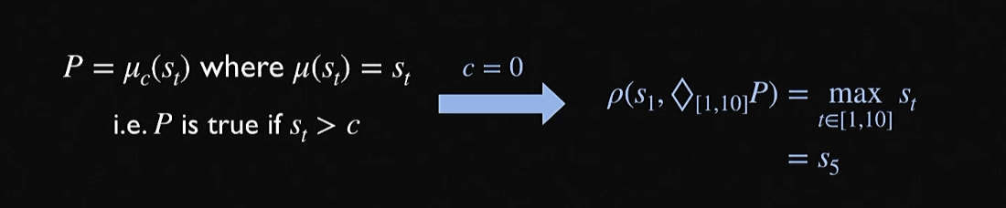
- allows us to specify properties over a time interval \(\qty [a, b]\), so we have \(\lozenge_{[a,b]} P\) (the “eventually” need to hold starting at \(a\) and until \(b\))
- allows us to to map real-valued signals to truth values \(\mu_{c}\qty(s_{t})\) is true if \(\mu\qty(s_{t}) > c\)
robustness (logic)
“robustness” is the amount by which achieve/miss a particular value; the bigger the magnitude, the “more” we did something; that is, very negative means super
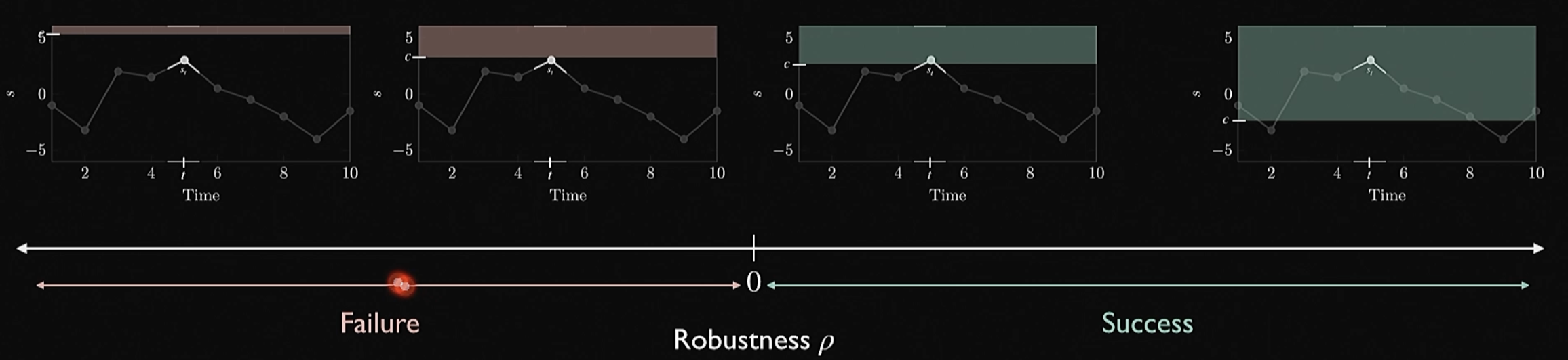
The above predicate could be computed for the formulae above using \(\rho \qty(s_{t}, P) = \mu_{t} \qty(s_{t}) - c\)
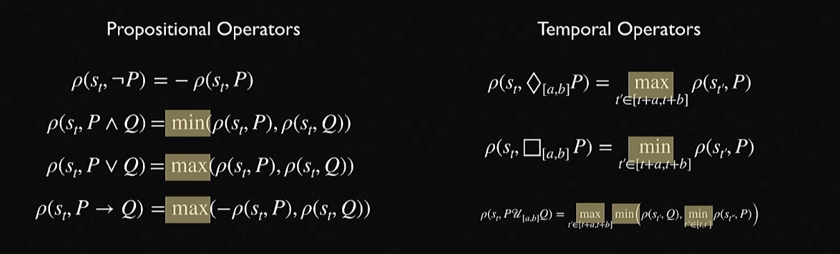
To calculate robustness to various predicates…
- \(\rho\qty(s_{t}, \neg P) = - \rho \qty(s_{t}, P)\)
- \(\rho\qty(s_{t}, P \wedge Q) = \min \qty(\rho \qty(s_{t}, P), \rho \qty(s_{t}, Q))\)
- \(\rho\qty(s_{t}, P \vee Q) = \max \qty(\rho \qty(s_{t}, P), \rho \qty(s_{t}, Q))\)
- \(\rho\qty(s_{t}, P \to Q) = \max \qty(-\rho \qty(s_{t}, P), \rho \qty(s_{t}, Q))\)
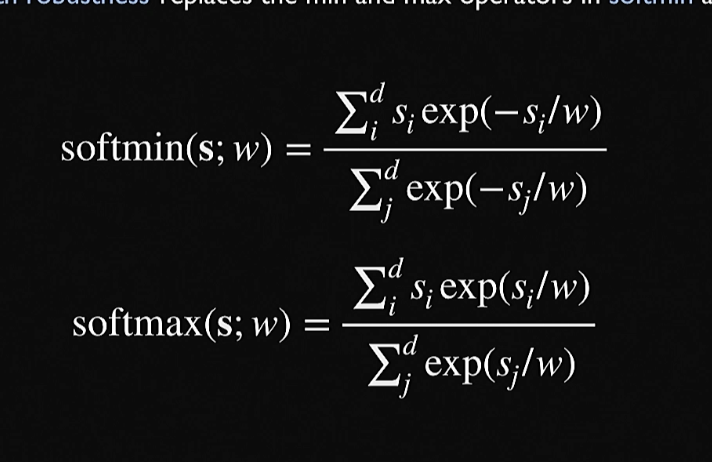
gradient of robustness
Binary values can’t be taken derivatives of. But, to take temporal derivatives, we instead take the softmin/softmax.