Insights to SVD: “ever matrix is a diagonal matrix, when viewed in the right space”
We can solve a linear system by moving it around:
\begin{align} Ac = b \\ \Rightarrow\ & U \Sigma V^{T} c = b \\ \Rightarrow\ & U \qty(\Sigma V^{T} c) = b \\ \Rightarrow\ & \Sigma V^{T} c = U^{T} b \end{align}
(since \(U\) is orthonormal, we can just flip it to invert it)
Call \(U^{T} b = \hat{b}\), call \(V^{T} c = \hat{c}\). We now have:
\begin{equation} \Sigma \hat{c} = \hat{b} \end{equation}
notice the very nice diagonal system we have here! Easy to solve. To get \(c\) back, we just write \(V \hat{c} = V \qty(V^{T} c) = c\).
Also, by noticing this, even during zero singular values, we can nicely identify where zero solutions/infinite solutions lie, etc. because
\begin{equation} \mqty(\sigma_{1} & 0 \\ 0 & \sigma_{2}) \mqty(c_1 \\ c_2) = \mqty(b_1 \\ b_2) \end{equation}
and we can like write \(b_1 = \sigma_{1} c_1\), \(b_2 = \sigma_{2} c_2\), and even if \(\sigma_{j}\) is \(0\), we can choose certain \(c\) that makes it work and claim the rest doesn’t work.
norms
Some norms:
\begin{equation} \Vert c \Vert_{1} = \sum_{k}^{}| c_{k}| \end{equation}
\begin{equation} \Vert c \Vert_{2} = \sqrt{\sum_{k}^{} c_{k}^{2}} \end{equation}
\begin{equation} \Vert c \Vert_{\infty} = \max_{k} | c_{k} | \end{equation}
Though they are theoretically sound, they are not all the same—not everything is “ok”. This is why the infinity norm is so important.
matrix norms
- \(\Vert A \Vert_{1}\) is the maximum absolute value column sum
- \(\Vert A \Vert_{\infty}\) is the maximum absolute value row sum
- \(\Vert A \Vert_{2}\) is the maximum eigenvalue of \(A^{T} A\) (that is, the maximum singular value of \(A\))
This means condition number….
\begin{equation} \Vert A \Vert_{2} \Vert A^{-1} \Vert_{2} \end{equation}
special matrices and their solvers
diagonal dominance
The magnitude of each diagonal element is…
- strictly larger than the sum of the magnitudens of all the other elements of eah row
- strictly larger than the sum of the magnitudes of all other elements in its column
If this is true, then, its:
- strictly diagonally dominant: matrix is non-singular
- column diagonal dominance: pivoting is not required during LU factorization
symmetric matrices
Since:
\begin{equation} A^{T} A = A A^{T} = A^{2} \end{equation}
so \(U\) and \(V\) may have the same eigenvectors. That is:
\begin{equation} A v_{k} = \sigma_{k} u_{k} \implies A v_{k} = \pm \sigma_{k} v_{k} \end{equation}
“if you are ok with your singular value to be flipped, you could use \(V\) for both \(U\) and \(V\)”. This is what we could write down:
\begin{equation} A = V \Lambda V^{T} \end{equation}
Whereby we could write down the eigenspaces of \(A\) directly:
\begin{equation} AV = V \Delta \end{equation}
We can convert a normal matrix to being “roughly symmetric” by writing:
\begin{equation} \hat{A} = \frac{1}{2} \qty(A + A^{T}) \end{equation}
also, inner product
see inner product, and in particular Matrix-scaled inner product
definiteness
- positive definite IFF \(v^{T} av > 0, \forall v \neq 0\)
- positive semi-definite IFF \(\langle v,v \rangle_{A} = V^{T} A v \geq 0, \forall v \neq 0\)
- negative definite IFF \(v^{T} A v < 0, \forall v \neq 0\)
- negative semi-definite: \(v^{T} A v \leq 0, \forall v \neq 0\)
Symmetric PD matricies: all eignevalues > 0 Symmetric PSD matricies: all EV >= 0
Positive definite: we can decompose the matrix into \(A = V\Sigma V^{T}\), if so, singular values are eigenvalues
SPSD has at least one \(\sigma_{k} = 0\) and a null space.
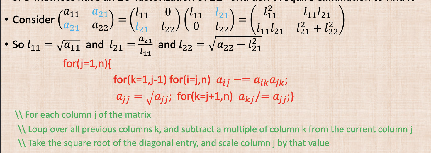
Cholesky Factorization
Symmetric Positive Definite matrix can be solved by factorizing into \(A = LL^{T}\).
Incomplete Cholesky PRedictioner
Cholesky Factorization can be used to conduct a preconditioner for a roughly sparse matrix.
Iterative Solvers
- direct solver: closed form strategy—special forms, sgaussian eliminations with LU, etc. etc.—but are closed forms so are very domain specific
- iterative solver: getting an initial guess, and then gradually improving the guess, terminate when the error is small